Basic examples
dummy.py
This is the most basic and simple example which generates randomized 256x256 images as fake detector events showing up as evt['photonPixelDetectors']['CCD'] for virtual events created at a repetition rate of 10 Hz:
import numpy as np

# Import analysis/plotting modules
from hummingbird import analysis, plotting

# Set new random seed
np.random.seed()

# Specify the facility
state = {}
state['Facility'] = 'Dummy'

# Create a dummy facility
state['Dummy'] = {
    # The event repetition rate of the dummy facility [Hz]
    'Repetition Rate' : 10,
    # Dictionary of data sources
    'Data Sources': {
        # The name of the data source.
        'CCD': {
            # A function that will generate the data for every event
            'data': lambda: np.random.rand(256,256),
            # The units to be used
            'unit': 'ADU',
            # The name of the category for this data source.
            # All data sources are aggregated by type, which is the key
            # used when asking for them in the analysis code.
            'type': 'photonPixelDetectors'
        }
    }
}

# This function is called for every single event
# following the given recipy of analysis
def onEvent(evt):

    # Processin rate [Hz]
    analysis.event.printProcessingRate()

    # Visualize detector image
    plotting.image.plotImage(evt['photonPixelDetectors']['CCD'], send_rate=10)
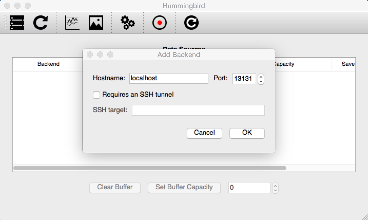
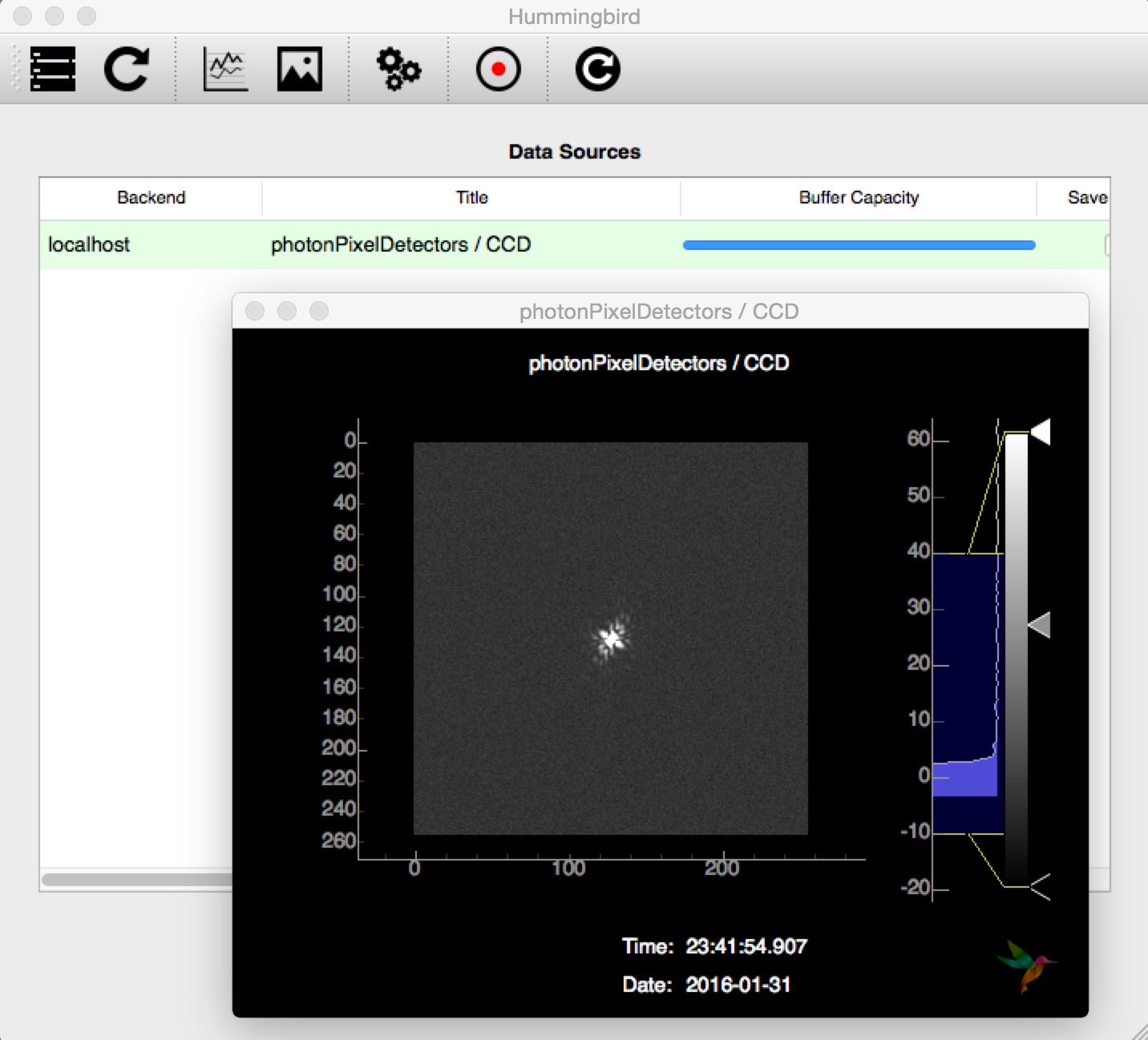
Notice that facility and data source is defined using the state variable. For every event, the current processing rate is printed and an image with the current virtual detector image is sent to the interface. Running this example in the backend (hummingbird.py -b examples/basic/dummy.py) we can start the frontend (hummingbird.py -i) in a separate shell (or even on a separate machine) and connect it to the backend by clicking on the left-most button:
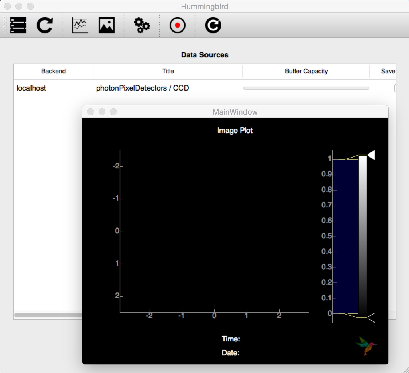
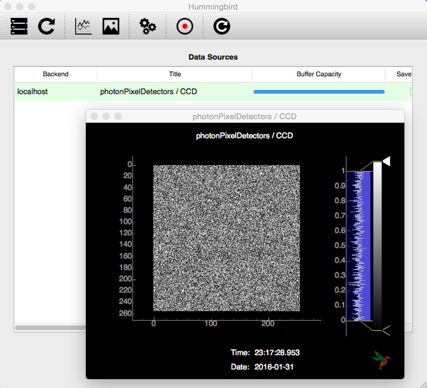
Once we are connecting, the virtual CCD shows up as a data source. After opening an image window (4th button from the left), we can subscribe to the CCD (menu Data sources) and the image that we were sending from the backend is displayed at a refreshing rate of 1 second:
simulation.py
For the next example, we replace the random detector images with CCD images that simulate diffraction from an object produced at a given hit rate (here 50%):
# Import analysis/plotting/simulation modules
from hummingbird import analysis, plotting, simulation

# Simulate diffraction data
sim = simulation.base.Simulation()
sim.hitrate = 0.5
sim.sigma = 1

# Specify the facility
state = {}
state['Facility'] = 'Dummy'

# Create a dummy facility
state['Dummy'] = {
    # The event repetition rate of the dummy facility [Hz]
    'Repetition Rate' : 10,
    # Specify simulation
    'Simulation': sim,
    # Dictionary of data sources
    'Data Sources': {
        # Data from a virtual diffraction detector
        'CCD': {
            # Fetch diffraction data from the simulation
            'data': sim.get_pattern,
            'unit': 'ADU',
            'type': 'photonPixelDetectors'
        }
    }
}

# This function is called for every single event
# following the given recipy of analysis
def onEvent(evt):

    # Processing rate [Hz]
    analysis.event.printProcessingRate()

    # Visualize detector image
    plotting.image.plotImage(evt['photonPixelDetectors']['CCD'], vmin=-10, vmax=40)
Following the same procedure as for dummy.py we can follow the hits (left) and misses (right) show up in the interface:
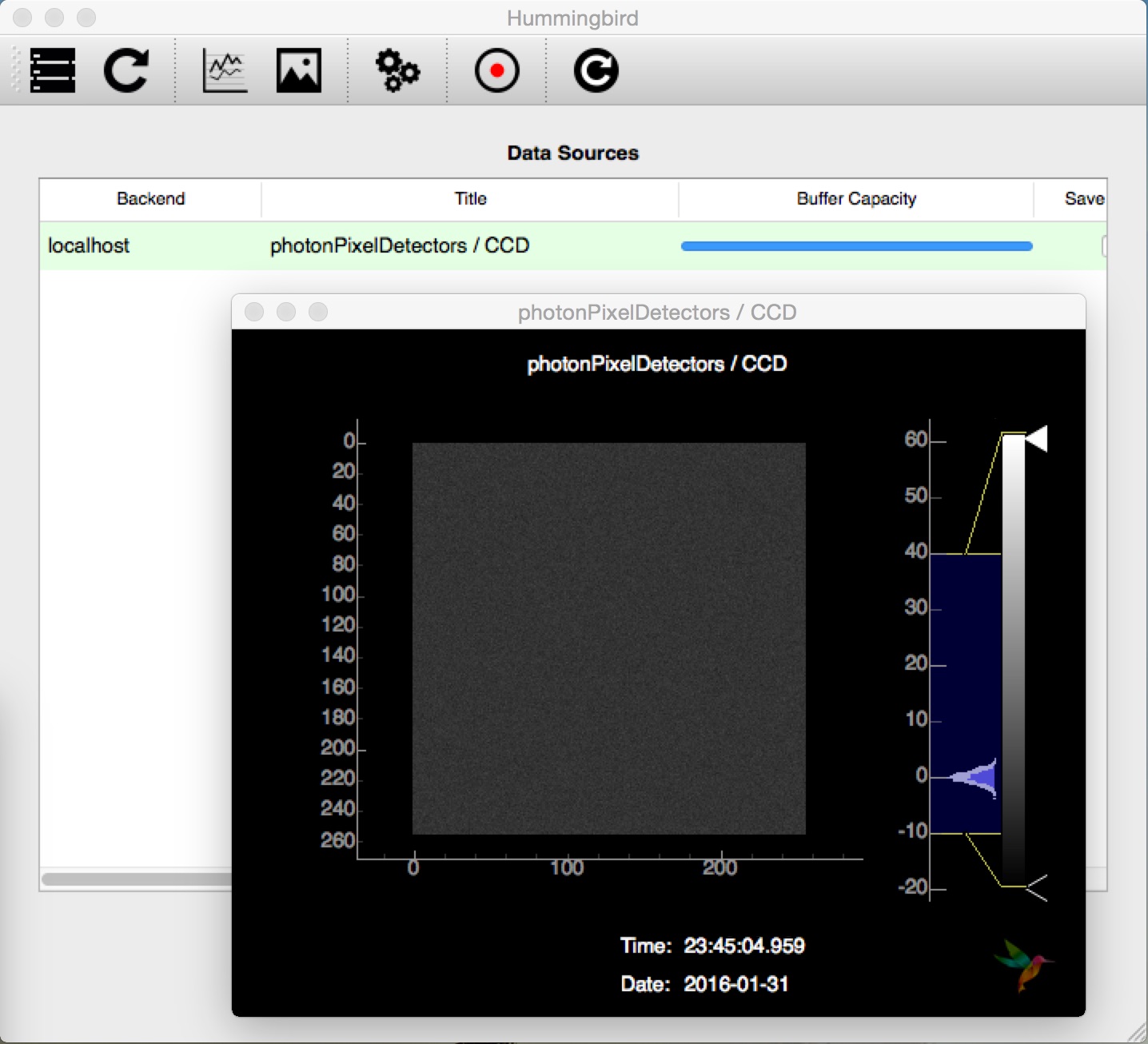
detector.py
In order to add more analysis of the detector we print some statistics, count the number of photons and send a history of the photon counts and per-event detector histograms along with the CCD image:
# Import analysis/plotting/simulation modules
from hummingbird import analysis, plotting, simulation

# Simulate diffraction data
sim = simulation.base.Simulation()
sim.hitrate = 0.5
sim.sigma = 1

# Specify the facility
state = {}
state['Facility'] = 'Dummy'

# Create a dummy facility
state['Dummy'] = {
    # The event repetition rate of the dummy facility [Hz]
    'Repetition Rate' : 10,
    # Specify simulation
    'Simulation': sim,
    # Dictionary of data sources
    'Data Sources': {
        # Data from a virtual diffraction detector
        'CCD': {
            # Fetch diffraction data from the simulation
            'data': sim.get_pattern,
            'unit': 'ADU',
            'type': 'photonPixelDetectors'
        }
    }
}

# Configuration for histogram plot
histogramCCD = {
    'hmin': -10,
    'hmax': 100,
    'bins': 200,
    'label': "Nr of photons",
    'history': 200}

# This function is called for every single event
# following the given recipy of analysis
def onEvent(evt):

    # Processing rate [Hz]
    analysis.event.printProcessingRate()

    # Detector statistics
    analysis.pixel_detector.printStatistics(evt["photonPixelDetectors"])

    # Count Nr. of Photons
    analysis.pixel_detector.totalNrPhotons(evt, evt["photonPixelDetectors"]["CCD"], outkey="nrPhotons")
    plotting.line.plotHistory(evt["analysis"]["nrPhotons"], label='Nr of photons / frame', history=50)

    # Detector histogram
    plotting.line.plotHistogram(evt["photonPixelDetectors"]["CCD"], **histogramCCD)

    # Detector images
    plotting.image.plotImage(evt["photonPixelDetectors"]["CCD"])
In the interface, we can now open a new line plot (3rd button from the left) and display the history of the photon counts by subscribing to the History(analysis/nrPhotons - CCD) data source:
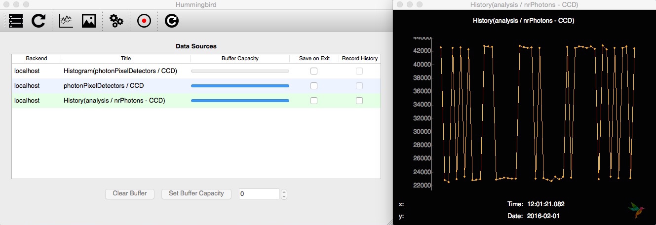
The depth of the history is defined by the length of the buffer, which can be resized in the main window. To the per-event histogram of the CCD we can subscribe both from an image plot (left panel) and from a line plot (right panel):
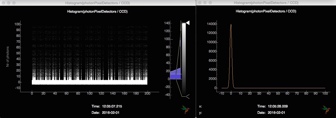
While the line plot shows the current histogram of the CCD, the image plot shows the history of the most recent detector histograms.
hitfinding.py
In the next example, we add htifinding to our analysis pipeline. We use a simply lit pixel counter given thresholds for the definition of a photon (aduThreshold=10) and for the definition of a hit (hitscoreThreshold=100):
# Import analysis/plotting/simulation modules
from hummingbird import analysis, plotting, simulation

# Simulate diffraction data
sim = simulation.base.Simulation()
sim.hitrate = 0.5
sim.sigma = 1

# Specify the facility
state = {}
state['Facility'] = 'Dummy'

# Create a dummy facility
state['Dummy'] = {
    # The event repetition rate of the dummy facility [Hz]
    'Repetition Rate' : 20,
    # Specify simulation
    'Simulation': sim,
    # Dictionary of data sources
    'Data Sources': {
        # Data from a virtual diffraction detector
        'CCD': {
            # Fetch diffraction data from the simulation
            'data': sim.get_pattern,
            'unit': 'ADU',
            'type': 'photonPixelDetectors'
        }
    }
}

# This function is called for every single event
# following the given recipy of analysis
def onEvent(evt):

    # Processing rate [Hz]
    analysis.event.printProcessingRate()

    # Simple hit finding (counting the number of lit pixels)
    analysis.hitfinding.countLitPixels(evt, evt["photonPixelDetectors"]["CCD"], aduThreshold=10, hitscoreThreshold=100)

    # Extract boolean (hit or miss)
    hit = evt["analysis"]["litpixel: isHit"].data

    # Compute the hitrate
    analysis.hitfinding.hitrate(evt, hit, history=5000)

    # Plot the hitscore
    plotting.line.plotHistory(evt["analysis"]["litpixel: hitscore"], label='Nr. of lit pixels', hline=100, group="A")

    # Plot the hitrate
    plotting.line.plotHistory(evt["analysis"]["hitrate"], label='Hit rate [%]', group="B")

    # Visualize detector image of hits
    if hit:
        plotting.image.plotImage(evt["photonPixelDetectors"]["CCD"], vmin=-10, vmax=40, group="Detectors")
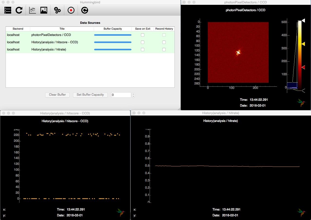
As compared to previos examples, we are plotting the CCD image only for hits. We are also sending history plots of hitscore and hitrate. The former can be very useful for finding the correct thresholds. When changing the threshold in the configuration file, there is no need to restart the backend. We can simply reload the configuration using the reload button (right-most button). Having all plots connected, the frontend looks like this:
correlation.py
In the last example, we show how it is possible to correlate and compare different parameters. Therefore, we first add more virtual data to our simulation: randomzied pulse energies and (x,y) injector positions. Along with plotting the history of pulse energies and plotting the correlation of pulse energy vs. hitscore as a scatter plot, we populate a map of averaged hitrates as a function the (x,y) injector position tuple:
# Import analysis/plotting/simulation modules
from hummingbird import analysis, plotting, simulation

# Simulate diffraction data
sim = simulation.base.Simulation()
sim.hitrate = 0.5
sim.sigma = 1

# Specify the facility
state = {}
state['Facility'] = 'Dummy'

# Create a dummy facility
state['Dummy'] = {
    # The event repetition rate of the dummy facility [Hz]
    'Repetition Rate' : 10,
    # Specify simulation
    'Simulation': sim,
    # Dictionary of data sources
    'Data Sources': {
        # Data from a virtual diffraction detector
        'CCD': {
            # Fetch diffraction data from the simulation
            'data': sim.get_pattern,
            'unit': 'ADU',
            'type': 'photonPixelDetectors'
        },
        # Data from a virutal pulse energy detector
        'pulseEnergy': {
            # Fetch pulse energy valus from the simulation
            'data': sim.get_pulse_energy,
            'unit': 'J',
            'type': 'pulseEnergies'
        },
        # Data from a virutal injector motor
        'injectorX': {
            # Fetch injector motor valus (x) from the simulation
            'data': sim.get_injector_x,
            'unit': 'm',
            'type': 'parameters'
        },
        # Data from a virutal injector motor
        'injectorY': {
            # Fetch injector motor valus (y) from the simulation
            'data': sim.get_injector_y,
            'unit': 'm',
            'type': 'parameters'
        }
    }
}

# Configuration for hitrate meanmap plot
hitmapParams = {
    'xmin':0,
    'xmax':1e-6,
    'ymin':0,
    'ymax':1e-6,
    'xbins':10,
    'ybins':10
}

# This function is called for every single event
# following the given recipy of analysis
def onEvent(evt):

    # Processing rate [Hz]
    analysis.event.printProcessingRate()

    # Simple hit finding (counting the number of lit pixels)
    analysis.hitfinding.countLitPixels(evt, evt["photonPixelDetectors"]["CCD"],
                                       aduThreshold=10, hitscoreThreshold=100)

    #analysis.beamline.averagePulseEnergy(evt, evt["pulseEnergies"])

    # Extract boolean (hit or miss)
    hit = evt["analysis"]["litpixel: isHit"].data

    # Compute the hitrate
    analysis.hitfinding.hitrate(evt, hit, history=1000)

    # Plot history of pulse energy
    plotting.line.plotHistory(evt['pulseEnergies']['pulseEnergy'])

    # Plot scatter of pulse energy vs. hitscore
    plotting.correlation.plotScatter(evt['pulseEnergies']['pulseEnergy'],
                                     evt["analysis"]["litpixel: hitscore"],
                                     xlabel='Pulse energy [J]', ylabel='Hitscore')

    # Plot heat map of hitrate as function of injector position
    plotting.correlation.plotMeanMap(evt["parameters"]['injectorX'], evt["parameters"]['injectorY'],
                                     evt["analysis"]["hitrate"].data, name='hitrateMeanMap', **hitmapParams)
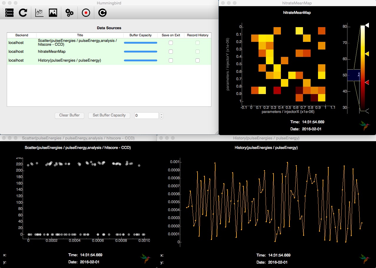
In the interface, these plots look like this: